You're reading the documentation of the v0.7. For the latest released version, please have a look at v0.11.

Boson Sampling with MPS

In this notebook, we explain how to use the MPS (Matrix Product State) backend to simulate a linear circuit. MPS simulation is based on a type of tensor network simulation, which gives an approximation of the output states [1] [2]. It does the computation on each component of the circuits one-by-one, and not on the whole unitary. The states are represented by tensors, which are then updated at each component. These tensors can be seen as a big set of matrices, and the approximation is done by chosing the dimension of these matrices, called the bond dimension. For this example, we simulate a simple boson sampling problem, with 6 modes and 3 photons [3].

import perceval as pcvl
import matplotlib.pyplot as plt

Definition of the circuit

Just like in the Boson Sampling notebook, we generate a Haar-random unitary and its decomposition in a circuit :

m = 6
unitary = pcvl.Matrix.random_unitary(m)
mzi = (pcvl.BS() // (0, pcvl.PS(phi=pcvl.Parameter("φ_a")))
       // pcvl.BS() // (1, pcvl.PS(phi=pcvl.Parameter("φ_b"))))
linear_circuit = pcvl.Circuit.decomposition(unitary, mzi,
                                               phase_shifter_fn=pcvl.PS,
                                               shape="triangle")

print(m, " modes triangular Boson Sampler :")
pcvl.pdisplay(linear_circuit, compact = True)

6  modes triangular Boson Sampler :

MPS simulation

Let us now define the MPS simulation, using the MPS backend in Perceval.

simulator_backend = pcvl.BackendFactory().get_backend("MPS")
simMPS = simulator_backend(linear_circuit)

We now choose the size of the matrices (the bond dimension) for our simulation.

chi = 8
simMPS.set_cutoff(chi)

And finally, we get the output probability distribution from a given input state with 3 photons.

n = 3
input_state = pcvl.BasicState([1]*n + [0]*(m-n))

probs = pcvl.BSDistribution({state : prob for state, prob in simMPS.allstateprob_iterator(input_state)})
pcvl.pdisplay(probs, max_v=20)

state	probability
|0,0,1,0,2,0>	0.069394
|0,0,2,0,1,0>	0.061578
|1,0,0,1,1,0>	0.059484
|0,1,0,1,0,1>	0.053757
|1,1,1,0,0,0>	0.042388
|0,0,0,2,1,0>	0.039433
|1,0,0,2,0,0>	0.039077
|0,2,0,1,0,0>	0.037225
|0,1,0,2,0,0>	0.031791
|0,1,1,0,1,0>	0.028824
|1,1,0,0,1,0>	0.028661
|0,0,3,0,0,0>	0.028538
|0,1,1,1,0,0>	0.024825
|2,0,0,0,1,0>	0.024031
|0,1,1,0,0,1>	0.022896
|0,1,2,0,0,0>	0.021384
|1,1,0,0,0,1>	0.021065
|0,1,0,0,1,1>	0.020496
|0,2,1,0,0,0>	0.020191
|0,0,0,3,0,0>	0.020153

Certification of the MPS method :

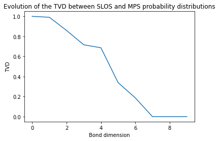
As we make an approximation by chosing the bond dimension, we have to check when does this approximation becomes good enough. Unfortunately, there is no formula giving the minimal size for a given approximation error. What we can do though is to compute the Total Variance Distance (TVD) between an ideal simulation of Boson Sampling, and an approximated one. To compute the ideal one, we can for instance use the SLOS backend on Perceval :

simulator_backend = pcvl.BackendFactory().get_backend("SLOS")
simSLOS = simulator_backend(unitary)

probsSLOS = pcvl.BSDistribution({state : prob for state, prob in simSLOS.allstateprob_iterator(input_state)})
pcvl.pdisplay(probs, max_v=20)

state	probability
|0,0,1,0,2,0>	0.069394
|0,0,2,0,1,0>	0.061578
|1,0,0,1,1,0>	0.059484
|0,1,0,1,0,1>	0.053757
|1,1,1,0,0,0>	0.042388
|0,0,0,2,1,0>	0.039433
|1,0,0,2,0,0>	0.039077
|0,2,0,1,0,0>	0.037225
|0,1,0,2,0,0>	0.031791
|0,1,1,0,1,0>	0.028824
|1,1,0,0,1,0>	0.028661
|0,0,3,0,0,0>	0.028538
|0,1,1,1,0,0>	0.024825
|2,0,0,0,1,0>	0.024031
|0,1,1,0,0,1>	0.022896
|0,1,2,0,0,0>	0.021384
|1,1,0,0,0,1>	0.021065
|0,1,0,0,1,1>	0.020496
|0,2,1,0,0,0>	0.020191
|0,0,0,3,0,0>	0.020153

We also have to define the TVD function.

def tvd(probs1, probs2):
    tvd = 0
    for state, prob in probs1.items():
        tvd += abs(prob - probs2[state])
    return tvd

Now we compute the TVD between the two simulations for different bond dimensions, going from 1 to 10.

TVD = []
for chi in range(1,11):
    simMPS.set_cutoff(chi)
    probsMPS = pcvl.BSDistribution({state : prob for state, prob in simMPS.allstateprob_iterator(input_state)})
    TVD += [tvd(probsMPS, probsSLOS)]

plt.plot(TVD)
plt.xlabel('Bond dimension')
plt.ylabel('TVD')
plt.title('Evolution of the TVD between SLOS and MPS probability distributions');

We can see that the TVD decreases as the size of the matrices increases, untill reaching 0 for a bond dimension of 7.

Annals of Physics, 326(1):96–192, jan 2011.

boson sampling using matrix product operators. Physical Review A, 104(2), aug 2021.

[3]: Hui Wang, et al. Boson Sampling with 20 Input Photons and a 60-Mode Interferometer in a \(10^{14}\)-Dimensional Hilbert Space. Physical Review Letters, 123(25):250503, December 2019. Publisher: American Physical Society.